Completed figures
Complete source
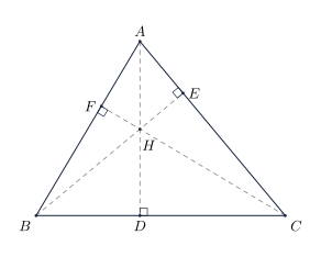
Altitude configuration
% Figure for a Classical Theorem Note
% Article: Two Views of the Orthocenter
% Site: Elementary Geometry
% Website: https://elementarygeometry.org/
% Drawing tool: tkz-euclide
% Output format: SVG
% Last verified: 2026-08-24
%
% Prepared for the web edition of this note.
%
% Editable source for public/diagrams/orthocenter-altitudes.svg.
% The production site serves the committed SVG and does not compile TeX.
\documentclass[tikz,border=8pt]{standalone}
\usepackage{tkz-euclide}

\definecolor{egNavy}{HTML}{17243D}
\definecolor{egGray}{HTML}{777671}
\definecolor{egRust}{HTML}{92513F}
\newcommand{\egUseStandardPlateAt}[1]{%
  \pgfresetboundingbox
  \path[use as bounding box]
    ([xshift=-102pt,yshift=-80pt]#1)
    rectangle
    ([xshift=102pt,yshift=80pt]#1);%
}
\newcommand{\egUseStandardPlate}{%
  \coordinate (egPlateCenter) at (current bounding box.center);%
  \egUseStandardPlateAt{egPlateCenter}%
}
\tikzset{
  eg figure/.style={line cap=round,line join=round,every node/.append style={font=\normalsize,text=egNavy}},
  eg main/.style={draw=egNavy,line width=0.75pt},
  eg support/.style={draw=egGray,line width=0.52pt},
  eg support dashed/.style={draw=egGray,line width=0.52pt,dash pattern=on 3pt off 3pt},
  eg accent/.style={draw=egRust,line width=0.75pt},
  eg mark/.style={draw=egNavy,line width=0.50pt}
}

\begin{document}
\begin{tikzpicture}[eg figure,scale=1.0]
  \tkzDefPoint(-0.5,4.2){A}
  \tkzDefPoint(-3,0){B}
  \tkzDefPoint(3,0){C}

  \tkzDefPointBy[projection=onto B--C](A)\tkzGetPoint{D}
  \tkzDefPointBy[projection=onto C--A](B)\tkzGetPoint{E}
  \tkzDefPointBy[projection=onto A--B](C)\tkzGetPoint{F}
  \tkzInterLL(B,E)(C,F)\tkzGetPoint{H}

  \tkzDrawSegments[eg support dashed](A,D B,E C,F)
  \tkzDrawSegments[eg main](A,B B,C C,A)

  \tkzMarkRightAngle[eg mark,size=0.18](A,D,C)
  \tkzMarkRightAngle[eg mark,size=0.18](B,E,A)
  \tkzMarkRightAngle[eg mark,size=0.18](C,F,B)

  \tkzDrawPoints[color=egNavy,fill=egNavy,size=1.6](A,B,C,D,E,F,H)
  \tkzLabelPoints[above](A)
  \tkzLabelPoints[below left](B)
  \tkzLabelPoints[below right](C)
  \tkzLabelPoints[below](D)
  \tkzLabelPoints[right](E)
  \tkzLabelPoints[left](F)
  \tkzLabelPoints[below right,xshift=-2pt,yshift=-4pt](H)
  \egUseStandardPlate
\end{tikzpicture}
\end{document}
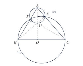
Cyclic-quadrilateral configuration
% Figure for a Classical Theorem Note
% Article: Two Views of the Orthocenter
% Site: Elementary Geometry
% Website: https://elementarygeometry.org/
% Drawing tool: tkz-euclide
% Output format: SVG
% Last verified: 2026-08-30
%
% Prepared for the web edition of this note.
%
% Editable source for public/diagrams/orthocenter-cyclic-proof.svg.
% The production site serves the committed SVG and does not compile TeX.
\documentclass[tikz,border=8pt]{standalone}
\usepackage{tkz-euclide}
\usetikzlibrary{angles,quotes}

\definecolor{egNavy}{HTML}{17243D}
\definecolor{egGray}{HTML}{777671}
\definecolor{egRust}{HTML}{92513F}
\newcommand{\egUseStandardPlateAt}[1]{%
  \pgfresetboundingbox
  \path[use as bounding box]
    ([xshift=-102pt,yshift=-80pt]#1)
    rectangle
    ([xshift=102pt,yshift=80pt]#1);%
}
\newcommand{\egUseStandardPlate}{%
  \coordinate (egPlateCenter) at (current bounding box.center);%
  \egUseStandardPlateAt{egPlateCenter}%
}
\tikzset{
  eg figure/.style={line cap=round,line join=round,every node/.append style={font=\normalsize,text=egNavy}},
  eg main/.style={draw=egNavy,line width=0.75pt},
  eg support/.style={draw=egGray,line width=0.52pt},
  eg support dashed/.style={draw=egGray,line width=0.52pt,dash pattern=on 3pt off 3pt},
  eg accent/.style={draw=egRust,line width=0.75pt},
  eg mark/.style={draw=egNavy,line width=0.50pt}
}

\begin{document}
\begin{tikzpicture}[eg figure,scale=1.0]
  % A compact configuration preserves the two cyclic quadrilaterals.
  \tkzDefPoint(-0.4,3.0){A}
  \tkzDefPoint(-2.2,0){B}
  \tkzDefPoint(2.2,0){C}
  \tkzDefPointBy[projection=onto A--C](B)\tkzGetPoint{E}
  \tkzDefPointBy[projection=onto A--B](C)\tkzGetPoint{F}
  \tkzInterLL(B,E)(C,F)\tkzGetPoint{H}
  \tkzInterLL(A,H)(B,C)\tkzGetPoint{D}

  \tkzDefCircle[circum](B,C,E)\tkzGetPoint{Oone}
  \tkzDefCircle[circum](A,E,F)\tkzGetPoint{Otwo}

  \tkzDrawCircle[eg main](Oone,B)
  \tkzDrawCircle[eg main](Otwo,A)
  \tkzDrawSegments[eg main](A,B B,C C,A)
  \tkzDrawSegments[eg support dashed](B,E C,F A,D)

  \tkzMarkRightAngle[eg mark,size=0.18](B,E,A)
  \tkzMarkRightAngle[eg mark,size=0.18](C,F,B)

  \tkzDrawPoints[color=egNavy,fill=egNavy,size=1.6](A,B,C,D,E,F,H)
  \tkzLabelPoint[above](A){$A$}
  \tkzLabelPoint[below left](B){$B$}
  \tkzLabelPoint[below right](C){$C$}
  \tkzLabelPoint[below](D){$D$}
  \tkzLabelPoint[above right](E){$E$}
  \tkzLabelPoint[above left](F){$F$}
  \tkzLabelPoint[below right](H){$H$}
  \node at (-2.1,-1.2) {$\omega_1$};
  \node at (1.2,2.6) {$\omega_2$};
  \egUseStandardPlate
\end{tikzpicture}
\end{document}
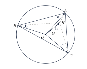
Vector and Euler-line configuration
% Figure for a Classical Theorem Note
% Article: Two Views of the Orthocenter
% Site: Elementary Geometry
% Website: https://elementarygeometry.org/
% Drawing tool: tkz-euclide
% Output format: SVG
% Last verified: 2026-08-30
%
% Prepared for the web edition of this note.
%
% Editable source for public/diagrams/orthocenter-vector-euler-line.svg.
% The production site serves the committed SVG and does not compile TeX.
\documentclass[tikz,border=8pt]{standalone}
\usepackage{tkz-euclide}
\usetikzlibrary{arrows.meta,calc}

\definecolor{egNavy}{HTML}{17243D}
\definecolor{egGray}{HTML}{777671}
\definecolor{egRust}{HTML}{92513F}
\newcommand{\egUseStandardPlateAt}[1]{%
  \pgfresetboundingbox
  \path[use as bounding box]
    ([xshift=-102pt,yshift=-80pt]#1)
    rectangle
    ([xshift=102pt,yshift=80pt]#1);%
}
\newcommand{\egUseStandardPlate}{%
  \coordinate (egPlateCenter) at (current bounding box.center);%
  \egUseStandardPlateAt{egPlateCenter}%
}
\tikzset{
  eg figure/.style={line cap=round,line join=round,every node/.append style={font=\normalsize,text=egNavy}},
  eg main/.style={draw=egNavy,line width=0.75pt},
  eg support/.style={draw=egGray,line width=0.52pt},
  eg support dashed/.style={draw=egGray,line width=0.52pt,dash pattern=on 3pt off 3pt},
  eg accent/.style={draw=egRust,line width=0.75pt},
  eg mark/.style={draw=egNavy,line width=0.50pt}
}

\begin{document}
\begin{tikzpicture}[eg figure,scale=1.0]
  % O is the origin. The three vertices are rotations of one radius point,
  % so their position vectors have exactly equal lengths.
  \tkzDefPoint(0,0){O}
  \tkzDefPoint(2.6,0){R}
  \tkzDefPointBy[rotation=center O angle 48](R)\tkzGetPoint{A}
  \tkzDefPointBy[rotation=center O angle 162](R)\tkzGetPoint{B}
  \tkzDefPointBy[rotation=center O angle -40](R)\tkzGetPoint{C}
  \tkzDefTriangleCenter[centroid](A,B,C)\tkzGetPoint{G}
  \tkzDefPointBy[homothety=center O ratio 3](G)\tkzGetPoint{H}

  \tkzDrawCircle[eg main](O,R)
  \tkzDrawSegments[eg main](A,B B,C C,A)
  \tkzDrawSegments[eg support dashed](A,H B,H C,H)
  \tkzDrawSegments[eg main,-{Latex[length=2.2mm,width=1.5mm]}](O,A O,B O,C)
  \tkzDrawSegment[eg main,-{Latex[length=2.2mm,width=1.5mm]}](O,H)

  \tkzDrawPoints[color=egNavy,fill=egNavy,size=1.6](A,B,C,O,G,H)
  \tkzLabelPoint[above](A){$A$}
  \tkzLabelPoint[left](B){$B$}
  \tkzLabelPoint[below right](C){$C$}
  \tkzLabelPoint[below left](O){$O$}
  \tkzLabelPoint[below right](G){$G$}
  \tkzLabelPoint[right](H){$H$}

  \node at ($(O)!0.7!(A)+(-0.1,0.2)$) {$\mathbf a$};
  \node at ($(O)!0.7!(B)+(0,0.2)$) {$\mathbf b$};
  \node at ($(O)!0.7!(C)+(0.1,0.2)$) {$\mathbf c$};
  \node at ($(O)!0.6!(H)+(0.2,-0.1)$) {$\mathbf h$};
  \egUseStandardPlate
\end{tikzpicture}
\end{document}