Completed figures
Complete source
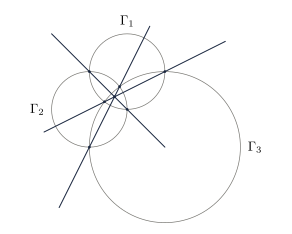
Three circles and their radical axes
% Figure for a Classical Theorem Note
% Article: Radical Axes and Orthogonal Parabolas
% Site: Elementary Geometry
% Website: https://elementarygeometry.org/
% Drawing tool: tkz-euclide
% Output format: SVG
% Last verified: 2026-08-30
% Accent target: none
%
% Editable source for public/diagrams/radical-axes-three-circles.svg.
% Prepared for the web edition of this note.
% The production site serves the committed SVG and does not compile TeX.
\documentclass[tikz,border=8pt]{standalone}
\usepackage{tkz-euclide}

\definecolor{egNavy}{HTML}{17243D}
\definecolor{egGray}{HTML}{777671}
\definecolor{egRust}{HTML}{92513F}

% Standard 5:4 figure plate.
% The standalone documents use border=8pt, so a 204pt by 160pt inner
% bounding box produces a 220pt by 176pt outer plate. Apply the plate only
% after every visible object and label has been drawn.
\newcommand{\egUseStandardPlateAt}[1]{%
  \pgfresetboundingbox
  \path[use as bounding box]
    ([xshift=-102pt,yshift=-80pt]#1)
    rectangle
    ([xshift=102pt,yshift=80pt]#1);%
}
\newcommand{\egUseStandardPlate}{%
  \coordinate (egPlateCenter) at (current bounding box.center);%
  \egUseStandardPlateAt{egPlateCenter}%
}

\tikzset{
  eg figure/.style={line cap=round,line join=round,every node/.append style={font=\normalsize,text=egNavy}},
  eg main/.style={draw=egNavy,line width=0.75pt},
  eg support/.style={draw=egGray,line width=0.52pt},
  eg support dashed/.style={draw=egGray,line width=0.52pt,dash pattern=on 3pt off 3pt},
  eg accent/.style={draw=egRust,line width=0.75pt},
  eg mark/.style={draw=egNavy,line width=0.50pt}
}

\begin{document}
\begin{tikzpicture}[eg figure,scale=1.0]
  % This is a quarter-turn of the original coordinate model.
  % Gamma_1: x^2+(y-1)^2=1.
  \tkzDefPoint(0,1){O1}
  \tkzDefPoint(0,2){U1}

  % Gamma_2: (x+1)^2+y^2=1.
  \tkzDefPoint(-1,0){O2}
  \tkzDefPoint(-2,0){U2}

  % Gamma_3: (x-1)^2+(y+1)^2=4.
  \tkzDefPoint(1,-1){O3}
  \tkzDefPoint(3,-1){U3}

  \tkzInterCC(O1,U1)(O2,U2)\tkzGetPoints{X12}{Y12}
  \tkzInterCC(O1,U1)(O3,U3)\tkzGetPoints{X13}{Y13}
  \tkzInterCC(O2,U2)(O3,U3)\tkzGetPoints{X23}{Y23}

  % The intersection is constructed from two independently defined radical axes.
  \tkzInterLL(X12,Y12)(X13,Y13)\tkzGetPoint{R}

  \tkzDrawCircle[eg support](O1,U1)
  \tkzDrawCircle[eg support](O2,U2)
  \tkzDrawCircle[eg support](O3,U3)

  \tkzDrawLine[eg main,add=1 and 1](X12,Y12)
  \tkzDrawLine[eg main,add=1 and 1](X13,Y13)
  \tkzDrawLine[eg main,add=1 and 1](X23,Y23)

  \tkzDrawPoints[color=egNavy,fill=egNavy,size=1.6](X12,Y12,X13,Y13,X23,Y23)
  \tkzDrawPoint[color=egNavy,fill=egNavy,size=1.6](R)

  \tkzLabelPoint[above,yshift=2pt](U1){$\Gamma_1$}
  \tkzLabelPoint[left,xshift=-2pt](U2){$\Gamma_2$}
  \tkzLabelPoint[right,xshift=2pt](U3){$\Gamma_3$}

  \egUseStandardPlate
\end{tikzpicture}
\end{document}
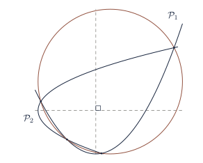
Perpendicular-axis parabolas and their common circle
% Figure for a Classical Theorem Note
% Article: Radical Axes and Orthogonal Parabolas
% Site: Elementary Geometry
% Website: https://elementarygeometry.org/
% Drawing tool: TikZ and tkz-euclide
% Output format: SVG
% Last verified: 2026-08-30
% Accent target: the circle through the four intersections
%
% Editable source for
% public/diagrams/orthogonal-parabolas-concyclic-intersections.svg.
% Prepared for the web edition of this note.
% The production site serves the committed SVG and does not compile TeX.
\documentclass[tikz,border=8pt]{standalone}
\usepackage{tkz-euclide}

\definecolor{egNavy}{HTML}{17243D}
\definecolor{egGray}{HTML}{777671}
\definecolor{egRust}{HTML}{92513F}

% Standard 5:4 figure plate.
% The standalone documents use border=8pt, so a 204pt by 160pt inner
% bounding box produces a 220pt by 176pt outer plate. Apply the plate only
% after every visible object and label has been drawn.
\newcommand{\egUseStandardPlateAt}[1]{%
  \pgfresetboundingbox
  \path[use as bounding box]
    ([xshift=-102pt,yshift=-80pt]#1)
    rectangle
    ([xshift=102pt,yshift=80pt]#1);%
}
\newcommand{\egUseStandardPlate}{%
  \coordinate (egPlateCenter) at (current bounding box.center);%
  \egUseStandardPlateAt{egPlateCenter}%
}

\tikzset{
  eg figure/.style={line cap=round,line join=round,every node/.append style={font=\normalsize,text=egNavy}},
  eg main/.style={draw=egNavy,line width=0.75pt},
  eg support/.style={draw=egGray,line width=0.52pt},
  eg support dashed/.style={draw=egGray,line width=0.52pt,dash pattern=on 3pt off 3pt},
  eg accent/.style={draw=egRust,line width=0.75pt},
  eg mark/.style={draw=egNavy,line width=0.50pt}
}

\begin{document}
\begin{tikzpicture}[eg figure,scale=1.0,x=1.1cm,y=1.1cm]
  % Eliminating y gives
  % x^4-6x^2-4x+1=(x+1)(x^3-x^2-5x+1)=0.
  % The trigonometric form below constructs the three cubic roots.
  \pgfmathsetmacro{\cubicangle}{acos(5/32)/3}
  \pgfmathsetmacro{\xA}{(1/3)+(8/3)*cos(\cubicangle-240)}
  \pgfmathsetmacro{\xB}{-1}
  \pgfmathsetmacro{\xC}{(1/3)+(8/3)*cos(\cubicangle-120)}
  \pgfmathsetmacro{\xD}{(1/3)+(8/3)*cos(\cubicangle)}
  \pgfmathsetmacro{\yA}{(\xA*\xA-1)/2}
  \pgfmathsetmacro{\yB}{(\xB*\xB-1)/2}
  \pgfmathsetmacro{\yC}{(\xC*\xC-1)/2}
  \pgfmathsetmacro{\yD}{(\xD*\xD-1)/2}
  \tkzDefPoint(\xA,\yA){A}
  \tkzDefPoint(\xB,\yB){B}
  \tkzDefPoint(\xC,\yC){C}
  \tkzDefPoint(\xD,\yD){D}

  \tkzDefPoint(0,1){O}
  \tkzDefPoint(1,1){X}
  \tkzDefPoint(0,2){Y}

  \draw[eg support dashed] (0,-0.5) -- (0,4.5);
  \draw[eg support dashed] (-2.1,1) -- (3.0,1);

  \draw[eg main,domain=-2.1:3.0,samples=161,variable=\t]
    plot ({\t},{(\t*\t-1)/2});
  \draw[eg main,domain=-0.5:3.2,samples=161,variable=\t]
    plot ({\t*\t-2*\t-1},{\t});

  % Adding the two parabola equations gives the circle below.
  \draw[eg accent] (0.5,2) circle[radius=2.5];

  \tkzMarkRightAngle[eg mark,size=0.18](X,O,Y)
  \tkzDrawPoints[color=egNavy,fill=egNavy,size=1.6](A,B,C,D)

  \node[above left,xshift=-1pt,yshift=1pt] at (3.0,4.0) {$\mathcal P_1$};
  \node[below left,xshift=-1pt,yshift=-1pt] at (-2.0,1.0) {$\mathcal P_2$};

  \egUseStandardPlate
\end{tikzpicture}
\end{document}